Rule of Succession - Mathematical Details

Mathematical Details

The proportion p is assigned a uniform distribution to describe the uncertainty about its true value. (Note: This proportion is not random, but uncertain. We assign a probability distribution to p to express our uncertainty, not to attribute randomness to p. But this amounts mathematically to the same thing as treating p as if it was random)

Let X_i is 1 if we observe a "success" on the ith trial, otherwise is 0, with probability p of success on each trial. Thus each X is 0 or 1; each X has a Bernoulli distribution. Suppose these Xs are conditionally independent given p.

Bayes' theorem says that in order to get the conditional probability distribution of p given the data X_i, i = 1, ..., n, one multiplies the "prior" (i.e., marginal) probability measure assigned to p by the likelihood function

where s = x₁ + ... + x_n is the number of "successes" and n is of course the number of trials, and then normalizes, to get the "posterior" (i.e., conditional on the data) probability distribution of p. (We are using capital X to denote a random variable and lower-case x either as the dummy in the definition of a function or as the data actually observed.)

The prior probability density function that expresses total ignorance of p except for the certain knowledge that it is neither 1 nor 0 (i.e., that we know that the experiment can in fact succeed or fail) is equal to 1 for 0 < p < 1 and equal to 0 otherwise. To get the normalizing constant, we find

(see beta function for more on integrals of this form).

The posterior probability density function is therefore

This is a beta distribution with expected value

Since the conditional probability for success in the next experiment, given the value of p, is just p, the law of total probability tell us that the probability of success in the next experiment is just the expected value of p. Since all of this is conditional on the observed data X_i for i = 1, ..., n, we have

The same calculation can be performed with the prior that expresses total ignorance of p, including ignorance with regards to the question whether the experiment can succeed, or can fail. This prior, except for a normalizing constant, is 1/(p(1 − p)) for 0 ≤ p ≤ 1 and 0 otherwise. If the calculation above is repeated with this prior, we get

Thus, with the prior specifying total ignorance, the probability of success is governed by the observed frequency of success. However, the posterior distribution which led to this result is the Beta(s,n − s) distribution, which will not be proper when s = n or s = 0 (i.e. the normalisation constant is infinite when s = 0 or s = n). This means that we cannot use this form of the posterior distribution to calculate the probability of the next observation being a success when s = 0 or s = n. This puts the information contained in the rule of succession in greater light: it can be thought of as expressing the prior assumption that if sampling was continued indefinitely, we would eventually observe at least one success, and at least one failure in the sample. The prior expressing total ignorance does not assume this knowledge.

To evaluate the "complete ignorance" case when s = 0 or s = n can be dealt with by first going back to the hypergeometric distribution, denoted by . This is the approach taken in Jaynes(2003). The binomial can be derived as a limiting form, where in such a way that their ratio remains fixed. One can think of as the number of successes in the total population, of size

The equivalent prior to is, with a domain of . Working conditional to means that estimating is equivalent to estimating, and then dividing this estimate by . The posterior for can be given as:

And it can be seen that, if ' = 'n or s = 0, then one of the factorials in the numerator will cancel exactly with one in the denominator. Taking the s = 0 case, we have:

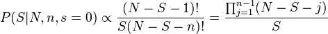
Adding in the normalising constant, which is always finite (because there is no singularities in the range of the posterior, and there are a finite number of terms) gives:

So the posterior expectation for is:

An approximate analytical expression for large N is given by first making the approximation to the product term:

and then replacing the summation in the numerator with an integral

The same procedure is followed for the denominator, but the process is a bit more tricky, as the integral is harder to evaluate

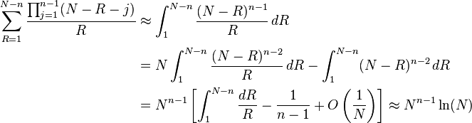
where ln is the natural logarithm plugging in these approximations into the expectation gives

where the base 10 logarithm has been used in the final answer for ease of calculation. For instance if the population is of size Nk then probability of success on the next sample is given by:

So for example, if the population be on the order of tens of billions, so that k = 10, and we observe n = 10 results without success, then the expected proportion in the population is approximately 0.43%. If the population is smaller, so that n = 10, k = 5 (tens of thousands), the expected proportion rises to approximately 0.86%, and so on. Similarly, if the number of observations is smaller, so that n = 5, k = 10, the proportion rise to approximately 0.86% again.

This probability has no lower bound, and can be made arbitrarily small for larger and larger choices of N, or k. This means that the probability depends on the size of the population from which one is sampling. In passing to the limit of infinite N (for the simpler analytic properties) we are "throwing away" a piece of very important information. Note that this ignorance relationship will only hold as long as only no successes are observed. It will be correspondingly revised straight back up to the observed frequency rule as soon as 1 success is observed. The corresponding results are found for the s=n case by switching labels, and then subtracting the probability from 1.