Normal Distribution - Estimation of Parameters

Estimation of Parameters

It is often the case that we don't know the parameters of the normal distribution, but instead want to estimate them. That is, having a sample (x₁, …, x_n) from a normal N(μ, σ2) population we would like to learn the approximate values of parameters μ and σ2. The standard approach to this problem is the maximum likelihood method, which requires maximization of the log-likelihood function:

$\ln\mathcal{L}(\mu,\sigma^2) = \sum_{i=1}^n \ln f(x_i;\,\mu,\sigma^2) = -\frac{n}{2}\ln(2\pi) - \frac{n}{2}\ln\sigma^2 - \frac{1}{2\sigma^2}\sum_{i=1}^n (x_i-\mu)^2.$

Taking derivatives with respect to μ and σ2 and solving the resulting system of first order conditions yields the maximum likelihood estimates:

$\hat{\mu} = \overline{x} \equiv \frac{1}{n}\sum_{i=1}^n x_i, \qquad \hat{\sigma}^2 = \frac{1}{n} \sum_{i=1}^n (x_i - \overline{x})^2.$

Estimator is called the sample mean, since it is the arithmetic mean of all observations. The statistic is complete and sufficient for μ, and therefore by the Lehmann–Scheffé theorem, is the uniformly minimum variance unbiased (UMVU) estimator. In finite samples it is distributed normally:

$\hat\mu \ \sim\ \mathcal{N}(\mu,\,\,\sigma^2\!\!\;/n).$

The variance of this estimator is equal to the μμ-element of the inverse Fisher information matrix . This implies that the estimator is finite-sample efficient. Of practical importance is the fact that the standard error of is proportional to, that is, if one wishes to decrease the standard error by a factor of 10, one must increase the number of points in the sample by a factor of 100. This fact is widely used in determining sample sizes for opinion polls and the number of trials in Monte Carlo simulations.

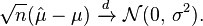
From the standpoint of the asymptotic theory, is consistent, that is, it converges in probability to μ as n → ∞. The estimator is also asymptotically normal, which is a simple corollary of the fact that it is normal in finite samples:

$\sqrt{n}(\hat\mu-\mu) \ \xrightarrow{d}\ \mathcal{N}(0,\,\sigma^2).$

The estimator is called the sample variance, since it is the variance of the sample (x₁, …, x_n). In practice, another estimator is often used instead of the . This other estimator is denoted s2, and is also called the sample variance, which represents a certain ambiguity in terminology; its square root s is called the sample standard deviation. The estimator s2 differs from by having (n − 1) instead of n in the denominator (the so called Bessel's correction):

$s^2 = \frac{n}{n-1}\,\hat\sigma^2 = \frac{1}{n-1} \sum_{i=1}^n (x_i - \overline{x})^2.$

The difference between s2 and becomes negligibly small for large n's. In finite samples however, the motivation behind the use of s2 is that it is an unbiased estimator of the underlying parameter σ2, whereas is biased. Also, by the Lehmann–Scheffé theorem the estimator s2 is uniformly minimum variance unbiased (UMVU), which makes it the "best" estimator among all unbiased ones. However it can be shown that the biased estimator is "better" than the s2 in terms of the mean squared error (MSE) criterion. In finite samples both s2 and have scaled chi-squared distribution with (n − 1) degrees of freedom:

$s^2 \ \sim\ \frac{\sigma^2}{n-1} \cdot \chi^2_{n-1}, \qquad \hat\sigma^2 \ \sim\ \frac{\sigma^2}{n} \cdot \chi^2_{n-1}\ .$

The first of these expressions shows that the variance of s2 is equal to 2σ4/(n−1), which is slightly greater than the σσ-element of the inverse Fisher information matrix . Thus, s2 is not an efficient estimator for σ2, and moreover, since s2 is UMVU, we can conclude that the finite-sample efficient estimator for σ2 does not exist.

Applying the asymptotic theory, both estimators s2 and are consistent, that is they converge in probability to σ2 as the sample size n → ∞. The two estimators are also both asymptotically normal:

$\sqrt{n}(\hat\sigma^2 - \sigma^2) \simeq \sqrt{n}(s^2-\sigma^2)\ \xrightarrow{d}\ \mathcal{N}(0,\,2\sigma^4).$

In particular, both estimators are asymptotically efficient for σ2.

By Cochran's theorem, for normal distribution the sample mean and the sample variance s2 are independent, which means there can be no gain in considering their joint distribution. There is also a reverse theorem: if in a sample the sample mean and sample variance are independent, then the sample must have come from the normal distribution. The independence between and s can be employed to construct the so-called t-statistic:

$t = \frac{\hat\mu-\mu}{s/\sqrt{n}} = \frac{\overline{x}-\mu}{\sqrt{\frac{1}{n(n-1)}\sum(x_i-\overline{x})^2}}\ \sim\ t_{n-1}$

This quantity t has the Student's t-distribution with (n − 1) degrees of freedom, and it is an ancillary statistic (independent of the value of the parameters). Inverting the distribution of this t-statistics will allow us to construct the confidence interval for μ; similarly, inverting the χ2 distribution of the statistic s2 will give us the confidence interval for σ2:

$\begin{align} & \mu \in \left[\, \hat\mu + t_{n-1,\alpha/2}\, \frac{1}{\sqrt{n}}s,\ \ \hat\mu + t_{n-1,1-\alpha/2}\,\frac{1}{\sqrt{n}}s \,\right] \approx \left[\, \hat\mu - |z_{\alpha/2}|\frac{1}{\sqrt n}s,\ \ \hat\mu + |z_{\alpha/2}|\frac{1}{\sqrt n}s \,\right], \\ & \sigma^2 \in \left[\, \frac{(n-1)s^2}{\chi^2_{n-1,1-\alpha/2}},\ \ \frac{(n-1)s^2}{\chi^2_{n-1,\alpha/2}} \,\right] \approx \left[\, s^2 - |z_{\alpha/2}|\frac{\sqrt{2}}{\sqrt{n}}s^2,\ \ s^2 + |z_{\alpha/2}|\frac{\sqrt{2}}{\sqrt{n}}s^2 \,\right], \end{align}$

where t_k,p and χ 2
k,p are the pth quantiles of the t- and χ2-distributions respectively. These confidence intervals are of the level 1 − α, meaning that the true values μ and σ2 fall outside of these intervals with probability α. In practice people usually take α = 5%, resulting in the 95% confidence intervals. The approximate formulas in the display above were derived from the asymptotic distributions of and s2. The approximate formulas become valid for large values of n, and are more convenient for the manual calculation since the standard normal quantiles z_α/2 do not depend on n. In particular, the most popular value of α = 5%, results in |z_0.025| = 1.96.

Read more about this topic: Normal Distribution

Famous quotes containing the words estimation and/or parameters:

“... it would be impossible for women to stand in higher estimation than they do here. The deference that is paid to them at all times and in all places has often occasioned me as much surprise as pleasure.”
—Frances Wright (1795–1852)

“What our children have to fear is not the cars on the highways of tomorrow but our own pleasure in calculating the most elegant parameters of their deaths.”
—J.G. (James Graham)