MUSCL Scheme - Linear Reconstruction

Linear Reconstruction

We will consider the fundamentals of the MUSCL scheme by considering the following simple first-order, scalar, 1D system, which is assumed to have a wave propagating in the positive direction,

Where represents a state variable and represents a flux variable.

The basic scheme of Godunov uses piecewise constant approximations for each cell, and results in a first-order upwind discretisation of the above problem with cell centres indexed as . A semi-discrete scheme can be defined as follows,

$\frac{d u_i}{d t} + \frac{1}{\Delta x_i} \left[ F \left( u_{i + 1} \right) - F \left( u_{i} \right) \right] =0.$

This basic scheme is not able to handle shocks or sharp discontinuities as they tend to become smeared. An example of this effect is shown in the diagram opposite, which illustrates a 1D advective equation with a step wave propagating to the right. The simulation was carried out with a mesh of 200 cells and used a 4th order Runge–Kutta time integrator (RK4).

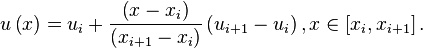
To provide higher resolution of discontinuities, Godunov's scheme can be extended to use piecewise linear approximations of each cell, which results in a central difference scheme that is second-order accurate in space. The piecewise linear approximations are obtained from

$u \left( x \right) = u_{i} + \frac{\left( x - x_{i} \right) }{ \left( x_{i+1} - x_{i} \right)} \left( u_{i+1} - u_{i} \right), x \in \left.$

Thus, evaluating fluxes at the cell edges we get the following semi-discrete scheme

$\frac{d u_i}{d t} + \frac{1}{\Delta x_i} \left[ F \left( u_{i + \frac{1}{2}} \right) - F \left( u_{i - \frac{1}{2}} \right) \right] =0,$

where and are the piecewise approximate values of cell edge variables, i.e.

Although the above second-order scheme provides greater accuracy for smooth solutions, it is not a total variation diminishing (TVD) scheme and introduces spurious oscillations into the solution where discontinuities or shocks are present. An example of this effect is shown in the diagram opposite, which illustrates a 1D advective equation, with a step wave propagating to the right. This loss of accuracy is to be expected due to Godunov's theorem. The simulation was carried out with a mesh of 200 cells and used RK4 for time integration.

MUSCL based numerical schemes extend the idea of using a linear piecewise approximation to each cell by using slope limited left and right extrapolated states. This results in the following high resolution, TVD discretisation scheme,

$\frac{d u_i}{d t} + \frac{1}{\Delta x_i} \left[ F \left( u^*_{i + \frac{1}{2}} \right) - F \left( u^*_{i - \frac{1}{2}} \right) \right] =0.$

Which, alternatively, can be written in the more succinct form,

$\frac{d u_i}{d t} + \frac{1}{\Delta x_i} \left[ F^*_{i + \frac{1}{2}} - F^*_{i - \frac{1}{2}} \right] =0.$

The numerical fluxes correspond to a nonlinear combination of first and second-order approximations to the continuous flux function.

The symbols and represent scheme dependent functions (of the limited extrapolated cell edge variables), i.e.

$u^*_{i + \frac{1}{2}} = u^*_{i + \frac{1}{2}} \left( u^L_{i + \frac{1}{2}}, u^R_{i + \frac{1}{2}} \right), u^*_{i - \frac{1}{2}} = u^*_{i - \frac{1}{2}} \left( u^L_{i - \frac{1}{2}}, u^R_{i - \frac{1}{2}} \right),$

and

$u^L_{i + \frac{1}{2}} = u_i + 0.5 \phi \left( r_i \right) \left( u_{i+1} - u_i \right), u^R_{i + \frac{1}{2}} = u_{i+1} - 0.5 \phi \left( r_{i+1} \right) \left( u_{i+2} - u_{i+1} \right),$

$u^L_{i - \frac{1}{2}} = u_{i-1} + 0.5 \phi \left( r_{i-1} \right) \left( u_i - u_{i-1} \right), u^R_{i - \frac{1}{2}} = u_i - 0.5 \phi \left( r_i \right) \left( u_{i+1} - u_i \right),$

The function is a limiter function that limits the slope of the piecewise approximations to ensure the solution is TVD, thereby avoiding the spurious oscillations that would otherwise occur around discontinuities or shocks - see Flux limiter section. The limiter is equal to zero when and is equal to unity when . Thus, the accuracy of a TVD discretization degrades to first order at local extrema, but tends to second order over smooth parts of the domain.

The algorithm is straight forward to implement. Once a suitable scheme for has been chosen, such as the Kurganov and Tadmor scheme (see below), the solution can proceed using standard numerical integration techniques.

Read more about this topic: MUSCL Scheme