MUSCL Scheme - Example: 1D Euler Equations

Example: 1D Euler Equations

For simplicity we consider the 1D case without heat transfer and without body force. Therefore, in conservation vector form, the general Euler equations reduce to

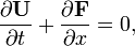
$\frac{\partial \mathbf{U}}{\partial t}+ \frac{\partial \mathbf{F}}{\partial x}=0,$

where

$\mathbf{U}=\begin{pmatrix}\rho \\ \rho u \\ E\end{pmatrix}\qquad \mathbf{F}=\begin{pmatrix}\rho u\\p+\rho u^2\\ u(E+p)\end{pmatrix},\qquad$

and where is a vector of states and is a vector of fluxes.

The equations above represent conservation of mass, momentum, and energy. There are thus three equations and four unknowns, (density) (fluid velocity), (pressure) and (total energy). The total energy is given by,

where represents specific internal energy.

In order to close the system an equation of state is required. One that suits our purpose is

where is equal to the ratio of specific heats for the fluid.

We can now proceed, as shown above in the simple 1D example, by obtaining the left and right extrapolated states for each state variable. Thus, for density we obtain

$\rho^*_{i + \frac{1}{2}} = \rho^*_{i + \frac{1}{2}} \left( \rho^L_{i + \frac{1}{2}}, \rho^R_{i + \frac{1}{2}} \right), \rho^*_{i - \frac{1}{2}} = \rho^*_{i - \frac{1}{2}} \left( \rho^L_{i - \frac{1}{2}}, \rho^R_{i - \frac{1}{2}} \right),$

where

$\rho^L_{i + \frac{1}{2}} = \rho_{i} + 0.5 \phi \left( r_{i} \right) \left( \rho_{i+1} - \rho_{i} \right), \rho^R_{i + \frac{1}{2}} = \rho_{i+1} - 0.5 \phi \left( r_{i+1} \right) \left( \rho_{i+2} - \rho_{i+1} \right),$

$\rho^L_{i - \frac{1}{2}} = \rho_{i-1} + 0.5 \phi \left( r_{i-1} \right) \left( \rho_{i} - \rho_{i-1} \right), \rho^R_{i - \frac{1}{2}} = \rho_{i} - 0.5 \phi \left( r_{i} \right) \left( \rho_{i+1} - \rho_{i} \right).$

Similarly, for momentum, and total energy . Velocity, is calculated from momentum, and pressure, is calculated from the equation of state.

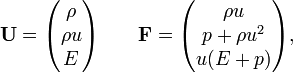
Having obtained the limited extrapolated states, we then proceed to construct the edge fluxes using these values. With the edge fluxes known, we can now construct the semi-discrete scheme, i.e.

$\frac{d \mathbf{U}_i}{d t} = - \frac{1}{\Delta x_i} \left[ \mathbf{F}^*_{i + \frac{1}{2} } - \mathbf{F}^*_{i - \frac{1}{2}} \right].$

The solution can now proceed by integration using standard numerical techniques.

The above illustrates the basic idea of the MUSCL scheme. However, for a practical solution to the Euler equations, a suitable scheme (such as the above KT scheme), also has to be chosen in order to define the function .

The diagram opposite shows a 2nd order solution to G A Sod's shock tube problem (Sod, 1978) using the above high resolution Kurganov and Tadmor Central Scheme (KT) with Linear Extrapolation and Ospre limiter. This illustrates clearly the effectiveness of the MUSCL approach to solving the Euler equations. The simulation was carried out on a mesh of 200 cells using Matlab code (Wesseling, 2001), adapted to use the KT algorithm and Ospre limiter. Time integration was performed by a 4th order SHK (equivalent performance to RK-4) integrator. The following initial conditions (SI units) were used:

pressure left = 100000 ;
pressure right= 10000 ;
density left = 1.0 ;
density right = 0.125 ;
length = 20 ;
velocity left = 0 ;
velocity right = 0 ;
duration =0.01 ;
lambda = 0.001069 (Δt/Δx).

The diagram opposite shows a 3rd order solution to G A Sod's shock tube problem (Sod, 1978) using the above high resolution Kurganov and Tadmor Central Scheme (KT) but with parabolic reconstruction and van Albada limiter. This again illustrates the effectiveness of the MUSCL approach to solving the Euler equations. The simulation was carried out on a mesh of 200 cells using Matlab code (Wesseling, 2001), adapted to use the KT algorithm with Parabolic Extrapolation and van Albada limiter. The alternative form of van Albada limiter, was used to avoid spurious oscillations. Time integration was performed by a 4th order SHK integrator. The same initial conditions were used.

Various other high resolution schemes have been developed that solve the Euler equations with good accuracy. Examples of such schemes are,

the Osher scheme, and
the Liou-Steffen AUSM (advection upstream splitting method) scheme.

More information on these and other methods can be found in the references below. An open source implementation of the Kurganov and Tadmor central scheme can be found in the external links below.

Read more about this topic: MUSCL Scheme