Fisher Information Metric - As Euclidean Metric

As Euclidean Metric

For a discrete probability space, that is, a probability space on a finite set of objects, the Fisher metric can be understood to simply be the flat Euclidean metric, after approriate changes of variable.

An N-dimensional sphere embedded in (N + 1)-dimensional space is defined as

The metric on the surface of the sphere is given by

where the are 1-forms; they are the basis vectors for the cotangent space. Writing as the basis vectors for the tangent space, so that, the Euclidean metric may be written as

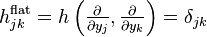
$h^\mathrm{flat}_{jk} = h\left(\tfrac{\partial}{\partial y_j}, \tfrac{\partial}{\partial y_k}\right) = \delta_{jk}$

The superscript 'flat' is there to remind that, when written in coordinate form, this metric is with respect to the flat-space coordinate . Consider now the change of variable . The sphere condition now becomes the probability normalization condition

while the metric becomes

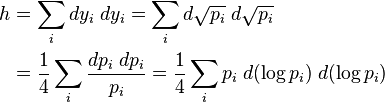
$\begin{align} h &=\sum_i dy_i \; dy_i = \sum_i d\sqrt{p_i} \; d\sqrt{p_i} \\ &= \frac{1}{4}\sum_i \frac{dp_i \; dp_i}{p_i} = \frac{1}{4}\sum_i p_i\; d(\log p_i) \; d(\log p_i) \end{align}$

The last can be recognized as one-fourth of the Fisher information metric. To complete the process, recall that the probabilities are parametric functions of the manifold variables, that is, one has . Thus, the above induces a metric on the parameter manifold:

$\begin{align} h & = \frac{1}{4}\sum_i p_i(\theta) \; d(\log p_i(\theta))\; d(\log p_i(\theta)) \\ &= \frac{1}{4}\sum_{jk} \sum_i p_i(\theta) \; \frac{\partial \log p_i(\theta)} {\partial \theta_j} \frac{\partial \log p_i(\theta)} {\partial \theta_k} d\theta_j d\theta_k \end{align}$

or, in coordinate form, the Fisher information metric is:

$\begin{align} g_{jk}(\theta) = 4h_{jk}^\mathrm{fisher} &= 4 h\left(\tfrac{\partial}{\partial \theta_j}, \tfrac{\partial}{\partial \theta_k}\right) \\ & = \sum_i p_i(\theta) \; \frac{\partial \log p_i(\theta)} {\partial \theta_j} \; \frac{\partial \log p_i(\theta)} {\partial \theta_k} \\ & = \mathrm{E}\left[ \frac{\partial \log p_i(\theta)} {\partial \theta_j} \; \frac{\partial \log p_i(\theta)} {\partial \theta_k} \right] \end{align}$

where, as before, . The superscript 'fisher' is present to remind that this expression is applicable for the coordinates ; whereas the non-coordinate form is the same as the Euclidean (flat-space) metric. That is, the Fisher information metric on a statistical manifold is simply (four times) the flat Euclidean metric, after appropriate changes of variable.

When the random variable is not discrete, but continuous, the argument still holds. This can be seen in one of two different ways. One way is to carefully recast all of the above steps in an infinite-dimensional space, being careful to define limits appropriately, etc., in order to make sure that all manipulations are well-defined, convergent, etc. The other way, as noted by Gromov, is to use a category-theoretic approach; that is, to note that the above manipulations remain valid in the category of probabilities.

Read more about this topic: Fisher Information Metric