Discrete Cosine Transform - Multidimensional DCTs

Multidimensional DCTs

Multidimensional variants of the various DCT types follow straightforwardly from the one-dimensional definitions: they are simply a separable product (equivalently, a composition) of DCTs along each dimension.

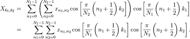
For example, a two-dimensional DCT-II of an image or a matrix is simply the one-dimensional DCT-II, from above, performed along the rows and then along the columns (or vice versa). That is, the 2d DCT-II is given by the formula (omitting normalization and other scale factors, as above):

Technically, computing a two- (or multi-) dimensional DCT by sequences of one-dimensional DCTs along each dimension is known as a row-column algorithm (after the two-dimensional case). As with multidimensional FFT algorithms, however, there exist other methods to compute the same thing while performing the computations in a different order (i.e. interleaving/combining the algorithms for the different dimensions).

The inverse of a multi-dimensional DCT is just a separable product of the inverse(s) of the corresponding one-dimensional DCT(s) (see above), e.g. the one-dimensional inverses applied along one dimension at a time in a row-column algorithm.

The image to the right shows combination of horizontal and vertical frequencies for an 8 x 8 two-dimensional DCT. Each step from left to right and top to bottom is an increase in frequency by 1/2 cycle. For example, moving right one from the top-left square yields a half-cycle increase in the horizontal frequency. Another move to the right yields two half-cycles. A move down yields two half-cycles horizontally and a half-cycle vertically. The source data (8x8) is transformed to a linear combination of these 64 frequency squares.