Tautochrone Curve - Abel's Solution

Abel's Solution

Niels Henrik Abel attacked a generalized version of the tautochrone problem (Abel's mechanical problem), namely, given a function T(y) that specifies the total time of descent for a given starting height, find an equation of the curve that yields this result. The tautochrone problem is a special case of Abel's mechanical problem when T(y) is a constant.

Abel's solution begins with the principle of conservation of energy — since the particle is frictionless, and thus loses no energy to heat, its kinetic energy at any point is exactly equal to the difference in potential energy from its starting point. The kinetic energy is, and since the particle is constrained to move along a curve, its velocity is simply, where is the distance measured along the curve. Likewise, the gravitational potential energy gained in falling from an initial height to a height is, thus:

$\begin{align} \frac{1}{2} m \left ( \frac{ds}{dt} \right ) ^2 & = mg(y_0-y) \\ \frac{ds}{dt} & = \pm \sqrt{2g(y_0-y)} \\ dt & = \pm \frac{ds}{\sqrt{2g(y_0-y)}} \\ dt & = - \frac{1}{\sqrt{2g(y_0-y)}} \frac{ds}{dy} \,dy \end{align}$

In the last equation, we've anticipated writing the distance remaining along the curve as a function of height (s(y)), recognized that the distance remaining must decrease as time increases (thus the minus sign), and used the chain rule in the form .

Now we integrate from to to get the total time required for the particle to fall:

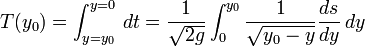
$T(y_0) = \int_{y=y_0}^{y=0} \, dt = \frac{1}{\sqrt{2g}} \int_0^{y_0} \frac{1}{\sqrt{y_0-y}} \frac{ds}{dy} \, dy$

This is called Abel's integral equation and allows us to compute the total time required for a particle to fall along a given curve (for which would be easy to calculate). But Abel's mechanical problem requires the converse — given, we wish to find, from which an equation for the curve would follow in a straightforward manner. To proceed, we note that the integral on the right is the convolution of with and thus take the Laplace transform of both sides:

$\mathcal{L} = \frac{1}{\sqrt{2g}} \mathcal{L} \left \mathcal{L} \left$

Since, we now have an expression for the Laplace transform of in terms of 's Laplace transform:

$\mathcal{L}\left = \sqrt{\frac{2g}{\pi}} z^{\frac{1}{2}} \mathcal{L}$

This is as far as we can go without specifying . Once is known, we can compute its Laplace transform, calculate the Laplace transform of and then take the inverse transform (or try to) to find .

For the tautochrone problem, is constant. Since the Laplace transform of 1 is, we continue:

$\begin{align} \mathcal{L}\left & = \sqrt{\frac{2g}{\pi}} z^{\frac{1}{2}} \mathcal{L} \\ & = \sqrt{\frac{2g}{\pi}} T_0 z^{-\frac{1}{2}} \end{align}$

Making use again of the Laplace transform above, we invert the transform and conclude:

$\frac{ds}{dy} = T_0 \frac{\sqrt{2g}}{\pi}\frac{1}{\sqrt{y}}$

It can be shown that the cycloid obeys this equation.

(Simmons, Section 54).

Read more about this topic: Tautochrone Curve

Famous quotes containing the word solution:

“There’s one solution that ends all life’s problems.”
—Chinese proverb.