Spherical Multipole Moments - Spherical Multipole Moments of A Point Charge

Spherical Multipole Moments of A Point Charge

The electric potential due to a point charge located at is given by

$\Phi(\mathbf{r}) = \frac{q}{4\pi\varepsilon} \frac{1}{R} = \frac{q}{4\pi\varepsilon} \frac{1}{\sqrt{r^{2} + r^{\prime 2} - 2 r^{\prime} r \cos \gamma}}.$

where is the distance between the charge position and the observation point and is the angle between the vectors and . If the radius of the observation point is greater than the radius of the charge, we may factor out 1/r and expand the square root in powers of using Legendre polynomials

$\Phi(\mathbf{r}) = \frac{q}{4\pi\varepsilon r} \sum_{l=0}^{\infty} \left( \frac{r^{\prime}}{r} \right)^{l} P_{l}(\cos \gamma )$

This is exactly analogous to the axial multipole expansion.

We may express in terms of the coordinates of the observation point and charge position using the spherical law of cosines (Fig. 2)

$\cos \gamma = \cos \theta \cos \theta^{\prime} + \sin \theta \sin \theta^{\prime} \cos(\phi - \phi^{\prime})$

Substituting this equation for into the Legendre polynomials and factoring the primed and unprimed coordinates yields the important formula known as the spherical harmonic addition theorem

$P_{l}(\cos \gamma) = \frac{4\pi}{2l + 1} \sum_{m=-l}^{l} Y_{lm}(\theta, \phi) Y_{lm}^{*}(\theta^{\prime}, \phi^{\prime})$

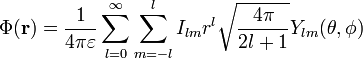
where the functions are the spherical harmonics. Substitution of this formula into the potential yields

$\Phi(\mathbf{r}) = \frac{q}{4\pi\varepsilon r} \sum_{l=0}^{\infty} \left( \frac{r^{\prime}}{r} \right)^{l} \left( \frac{4\pi}{2l+1} \right) \sum_{m=-l}^{l} Y_{lm}(\theta, \phi) Y_{lm}^{*}(\theta^{\prime}, \phi^{\prime})$

which can be written as

$\Phi(\mathbf{r}) = \frac{1}{4\pi\varepsilon} \sum_{l=0}^{\infty} \sum_{m=-l}^{l} \left( \frac{Q_{lm}}{r^{l+1}} \right) \sqrt{\frac{4\pi}{2l+1}} Y_{lm}(\theta, \phi)$

where the multipole moments are defined

$Q_{lm} \ \stackrel{\mathrm{def}}{=}\ q \left( r^{\prime} \right)^{l} \sqrt{\frac{4\pi}{2l+1}} Y_{lm}^{*}(\theta^{\prime}, \phi^{\prime})$ .

As with axial multipole moments, we may also consider the case when the radius of the observation point is less than the radius of the charge. In that case, we may write

$\Phi(\mathbf{r}) = \frac{q}{4\pi\varepsilon r^{\prime}} \sum_{l=0}^{\infty} \left( \frac{r}{r^{\prime}} \right)^{l} \left( \frac{4\pi}{2l+1} \right) \sum_{m=-l}^{l} Y_{lm}(\theta, \phi) Y_{lm}^{*}(\theta^{\prime}, \phi^{\prime})$

which can be written as

$\Phi(\mathbf{r}) = \frac{1}{4\pi\varepsilon} \sum_{l=0}^{\infty} \sum_{m=-l}^{l} I_{lm} r^{l} \sqrt{\frac{4\pi }{2l+1}} Y_{lm}(\theta, \phi)$

where the interior spherical multipole moments are defined as the complex conjugate of irregular solid harmonics

$I_{lm} \ \stackrel{\mathrm{def}}{=}\ \frac{q}{\left( r^{\prime} \right)^{l+1}} \sqrt{\frac{4\pi }{2l+1}} Y_{lm}^{*}(\theta^{\prime}, \phi^{\prime})$

The two cases can be subsumed in a single expression if and are defined to be the lesser and greater, respectively, of the two radii and ; the potential of a point charge then takes the form, which is sometimes referred to as Laplace expansion

$\Phi(\mathbf{r}) = \frac{q}{4\pi\varepsilon} \sum_{l=0}^{\infty} \frac{r_<^{l}}{r_>^{l+1}} \left( \frac{4\pi}{2l+1} \right) \sum_{m=-l}^{l} Y_{lm}(\theta, \phi) Y_{lm}^{*}(\theta^{\prime}, \phi^{\prime})$

Read more about this topic: Spherical Multipole Moments

Famous quotes containing the words moments, point and/or charge:

“It is time to provide a smashing answer for those cynical men who say that a democracy cannot be honest, cannot be efficient.... We have in the darkest moments of our national trials retained our faith in our own ability to master our own destiny.”
—Franklin D. Roosevelt (1882–1945)

“The women’s liberation movement at this point in history makes the American Communist Party of the 1930s look like a monolith.”
—Nora Ephron (b. 1941)

“The most serious charge which can be brought against New England is not Puritanism but February.”
—Joseph Wood Krutch (1893–1970)