Poynting Vector - Time-averaged Poynting Vector

Time-averaged Poynting Vector

For time-periodic sinusoidal electromagnetic fields, the average power flow per unit time is often more useful, and can be found by treating the electric and magnetic fields as complex vectors as follows (star * denotes the complex conjugate):

$\begin{align}\mathbf{S} & = \mathbf{E} \times \mathbf{H}\\ & = \mathrm{Re}\left(\mathbf{\widetilde E}\right) \times \mathrm{Re}\left(\mathbf{\widetilde H} \right)\\ & = \mathrm{Re}\left(\mathbf{E_c} e^{j\omega t}\right) \times \mathrm{Re}\left(\mathbf{H_c} e^{j\omega t}\right)\\ & = \frac{1}{2}\left(\mathbf{E_c} e^{j\omega t} + \mathbf{E_c}^* e^{-j\omega t}\right) \times \frac{1}{2}\left(\mathbf{H_c} e^{j\omega t} + \mathbf{H_c}^* e^{-j\omega t}\right)\\ & = \frac{1}{4}\left(\mathbf{E_c} \times \mathbf{H_c}^* + \mathbf{E_c}^* \times \mathbf{H_c} + \mathbf{E_c} \times \mathbf{H_c} e^{2j\omega t} + \mathbf{E_c}^* \times \mathbf{H_c}^* e^{-2j\omega t}\right)\\ & = \frac{1}{4}\left(\mathbf{E_c} \times \mathbf{H_c}^* + \left(\mathbf{E_c} \times \mathbf{H_c}^*\right)^* + \mathbf{E_c} \times \mathbf{H_c} e^{2j\omega t} + \left(\mathbf{E_c} \times \mathbf{H_c} e^{2j\omega t}\right)^*\right)\\ & = \frac{1}{2}\mathrm{Re}\left(\mathbf{E_c} \times \mathbf{H_c}^*\right) + \frac{1}{2}\mathrm{Re}\left(\mathbf{E_c} \times \mathbf{H_c} e^{2j\omega t}\right). \end{align}$

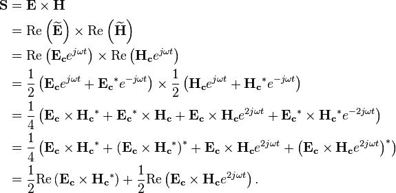
The average over time is given as

The second term is a sinusoidal curve

and its average is zero, giving

$\langle\mathbf{S}\rangle = \frac{1}{2}\mathrm{Re}\left(\mathbf{E_c} \times \mathbf{H_c}^*\right) =\frac{1}{2}\mathrm{Re}\left(\left \times \left\right) =\frac{1}{2}\mathrm{Re}\left(\mathbf{\widetilde E} \times \mathbf{\widetilde H}^*\right).$

Read more about this topic: Poynting Vector