Motivating Example
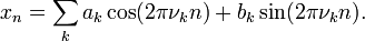
Suppose, from to is a time series (discrete time) with zero mean. Suppose that it is a sum of a finite number of periodic components (all frequencies are positive):
The variance of is, by definition, . If these data were samples taken from an electrical signal, this would be its average power (power is energy per unit time, so it is analogous to variance if energy is analogous to the amplitude squared).
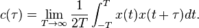
Now, for simplicity, suppose the signal extends infinitely in time, so we pass to the limit as . If the average power is bounded, which is almost always the case in reality, then the following limit exists and is the variance of the data.

Again, for simplicity, we will pass to continuous time, and assume that the signal extends infinitely in time in both directions. Then these two formulas become

and

But obviously the root mean square of either or is, so the variance of is and that of is . Hence, the power of which comes from the component with frequency is . All these contributions add up to the power of .
Then the power as a function of frequency is obviously, and its statistical cumulative distribution function will be
is a step function, monotonically non-decreasing. Its jumps occur at the the frequencies of the periodic components of, and the value of each jump is the power or variance of that component.
The variance is the covariance of the data with itself. If we now consider the same data but with a lag of, we can take the covariance of with, and define this to be the autocorrelation function of the signal (or data) :
When it exists, it is an even function of . If the average power is bounded, then exists everywhere, is finite, and is bounded by, which is the power or variance of the data.
It is elementary to show that can be decomposed into periodic components with the same periods as :

This is in fact the spectral decomposition of over the different frequencies, and is obviously related to the distribution of power of over the frequencies: the amplitude of a frequency component of is its contribution to the power of the signal.
Read more about this topic: Spectral Density
Famous quotes containing the word motivating:
“Decisive inventions and discoveries always are initiated by an intellectual or moral stimulus as their actual motivating force, but, usually, the final impetus to human action is given by material impulses ... merchants stood as a driving force behind the heroes of the age of discovery; this first heroic impulse to conquer the world emanated from very mortal forces—in the beginning, there was spice.”
—Stefan Zweig (18811942)
“...one of my motivating forces has been to recreate the world I know into a world I wish I could be in. Hence my optimism and happy endings. But I’ve never dreamed I could actually reshape the real world.”
—Kristin Hunter (b. 1931)