Maximum Likelihood - Properties - Asymptotic Normality

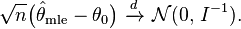
Asymptotic Normality

Maximum-likelihood estimators can lack asymptotic normality and can be inconsistent if there is a failure of one (or more) of the below regularity conditions:

Estimate on boundary. Sometimes the maximum likelihood estimate lies on the boundary of the set of possible parameters, or (if the boundary is not, strictly speaking, allowed) the likelihood gets larger and larger as the parameter approaches the boundary. Standard asymptotic theory needs the assumption that the true parameter value lies away from the boundary. If we have enough data, the maximum likelihood estimate will keep away from the boundary too. But with smaller samples, the estimate can lie on the boundary. In such cases, the asymptotic theory clearly does not give a practically useful approximation. Examples here would be variance-component models, where each component of variance, σ2, must satisfy the constraint σ2 ≥0.

Data boundary parameter-dependent. For the theory to apply in a simple way, the set of data values which has positive probability (or positive probability density) should not depend on the unknown parameter. A simple example where such parameter-dependence does hold is the case of estimating θ from a set of independent identically distributed when the common distribution is uniform on the range (0,θ). For estimation purposes the relevant range of θ is such that θ cannot be less than the largest observation. Because the interval (0,θ) is not compact, there exists no maximum for the likelihood function: For any estimate of theta, there exists a greater estimate that also has greater likelihood. In contrast, the interval includes the end-point θ and is compact, in which case the maximum-likelihood estimator exists. However, in this case, the maximum-likelihood estimator is biased. Asymptotically, this maximum-likelihood estimator is not normally distributed.

Nuisance parameters. For maximum likelihood estimations, a model may have a number of nuisance parameters. For the asymptotic behaviour outlined to hold, the number of nuisance parameters should not increase with the number of observations (the sample size). A well-known example of this case is where observations occur as pairs, where the observations in each pair have a different (unknown) mean but otherwise the observations are independent and Normally distributed with a common variance. Here for 2N observations, there are N+1 parameters. It is well known that the maximum likelihood estimate for the variance does not converge to the true value of the variance.

Increasing information. For the asymptotics to hold in cases where the assumption of independent identically distributed observations does not hold, a basic requirement is that the amount of information in the data increases indefinitely as the sample size increases. Such a requirement may not be met if either there is too much dependence in the data (for example, if new observations are essentially identical to existing observations), or if new independent observations are subject to an increasing observation error.

Some regularity conditions which ensure this behavior are:

1. The first and second derivatives of the log-likelihood function must be defined.
2. The Fisher information matrix must not be zero, and must be continuous as a function of the parameter.
3. The maximum likelihood estimator is consistent.

Suppose that conditions for consistency of maximum likelihood estimator are satisfied, and

1. θ₀ ∈ interior(Θ);
2. f(x|θ) > 0 and is twice continuously differentiable in θ in some neighborhood N of θ₀;
3. ∫ sup_θ∈N||∇_θf(x|θ)||dx < ∞, and ∫ sup_θ∈N||∇_θθf(x|θ)||dx < ∞;
4. I = E exists and is nonsingular;
5. E < ∞.

Then the maximum likelihood estimator has asymptotically normal distribution:

Proof, skipping the technicalities:

Since the log-likelihood function is differentiable, and θ₀ lies in the interior of the parameter set, in the maximum the first-order condition will be satisfied:

When the log-likelihood is twice differentiable, this expression can be expanded into a Taylor series around the point θ = θ₀:

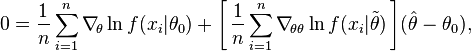
where is some point intermediate between θ₀ and . From this expression we can derive that

Here the expression in square brackets converges in probability to H = E by the law of large numbers. The continuous mapping theorem ensures that the inverse of this expression also converges in probability, to H−1. The second sum, by the central limit theorem, converges in distribution to a multivariate normal with mean zero and variance matrix equal to the Fisher information I. Thus, applying the Slutsky's theorem to the whole expression, we obtain that

Finally, the information equality guarantees that when the model is correctly specified, matrix H will be equal to the Fisher information I, so that the variance expression simplifies to just I−1.