Extended Kalman Filter - Discrete-time Extended Kalman Filter

Discrete-time Extended Kalman Filter

Most physical systems are represented as continuous-time models while discrete-time measurements are frequently taken for state estimation via a digital processor. Therefore, the system model and measurement model are given by

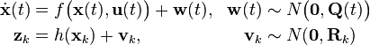
$\begin{align} \dot{\mathbf{x}}(t) &= f\bigl(\mathbf{x}(t), \mathbf{u}(t)\bigr) + \mathbf{w}(t), &\mathbf{w}(t) &\sim N\bigl(\mathbf{0},\mathbf{Q}(t)\bigr) \\ \mathbf{z}_k &= h(\mathbf{x}_k) + \mathbf{v}_k, &\mathbf{v}_k &\sim N(\mathbf{0},\mathbf{R}_k) \end{align}$

where .

Initialize

$\hat{\mathbf{x}}_{0|0}=E\bigl, \mathbf{P}_{0|0}=Var\bigl$

Predict

$\begin{align} &\begin{cases} \dot{\hat{\mathbf{x}}}(t) = f\bigl(\hat{\mathbf{x}}(t), \mathbf{u}(t)\bigr), \\ \dot{\mathbf{P}}(t) = \mathbf{F}(t)\mathbf{P}(t)+\mathbf{P}(t)\mathbf{F}(t)^\top + \mathbf{Q}(t), \end{cases}\qquad \text{with } \begin{cases} \hat{\mathbf{x}}(t_{k-1}) = \hat{\mathbf{x}}_{k-1|k-1}, \\ \mathbf{P}(t_{k-1}) = \mathbf{P}_{k-1|k-1}, \end{cases} \\ \Rightarrow &\begin{cases} \hat{\mathbf{x}}_{k|k-1} = \hat{\mathbf{x}}(t_k) \\ \mathbf{P}_{k|k-1} = \mathbf{P}(t_k) \end{cases} \end{align}$

where

Update

where

The update equations are identical to those of discrete-time extended Kalman filter.

Read more about this topic: Extended Kalman Filter

Famous quotes containing the word extended:

“Only very slowly and late have men come to realize that unless freedom is universal it is only extended privilege.”
—Christopher Hill (b. 1912)