Dirichlet Process - Introduction

Introduction

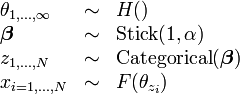
Consider a simple mixture model:

$\begin{array}{lcl} \theta_{1,\dots,K} &\sim& H \\ \boldsymbol\beta &\sim& \operatorname{Dirichlet}(\alpha/K,..., \alpha/K) \\ z_{1,\dots,N} &\sim& \operatorname{Categorical}(\boldsymbol\beta) \\ x_{i=1,\dots,N} &\sim& F(\theta_{z_i}) \end{array}$

This is a basic generative model where the observations are distributed according to a mixture of components, where each component is distributed according to a single parametric family but where different components have different values of, which is drawn in turn from a distribution . Typically, will be the conjugate prior distribution of . In addition, the prior probability of each component is specified by, which is a size- vector of probabilities, all of which add up to 1.

For example, if the observations are apartment prices and the components represent different neighborhoods, then might be a Gaussian distribution with unknown mean and unknown variance, with the mean and variance specifying the distribution of prices in that neighborhood. Then the parameter will be a vector of two values, a mean drawn from a Gaussian distribution and a variance drawn from an inverse gamma distribution, which are the conjugate priors of the mean and variance, respectively, of a Gaussian distribution.

Meanwhile, if the observations are words and the components represent different topics, then might be a categorical distribution over a vocabulary of size, with unknown frequencies of each word in the vocabulary, specifying the distribution of words in each particular topic. Then the parameter will be a vector of values, each representing a probability and all summing to one, drawn from a Dirichlet distribution, which is the conjugate prior of the categorical distribution.

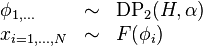
Now imagine we consider the limit as . Conceptually this means that we have no idea how many components are present. The result will be as follows:

$\begin{array}{lcl} \theta_{1,\dots,\infty} &\sim& H \\ \boldsymbol\beta &\sim& \operatorname{Stick}(1,\alpha) \\ z_{1,\dots,N} &\sim& \operatorname{Categorical}(\boldsymbol\beta) \\ x_{i=1,\dots,N} &\sim& F(\theta_{z_i}) \end{array}$

In this model, conceptually speaking there are an infinite number of components, each with a separate parameter value, and a correspondingly infinite number of prior probabilities for each component, drawn from a stick-breaking process (see section below). Note that a practical application of such a model would not actually store an infinite number of components. Instead, it would generate the component prior probabilities one at a time from the stick-breaking process, which by construction tends to return the largest probability values first. As each component probability is drawn, a corresponding parameter value is also drawn. At any one time, some of the prior probability mass will be assigned to components and some unassigned. To generate a new observation, a random number between 0 and 1 is drawn uniformly, and if it lands in the unassigned mass, new components are drawn as necessary (each one reducing the amount of unassigned mass) until enough mass has been allocated to place this number in an existing component. Each time a new component probability is generated by the stick-breaking process, a corresponding parameter value is drawn from .

Sometimes, the stick-breaking process is denoted as, after the authors of this process, instead of .

Another view of this model comes from looking back at the finite-dimensional mixture model with mixing probabilities drawn from a Dirichlet distribution and considering the distribution of a particular component assignment conditioned on all previous components, with the mixing probabilities integrated out. This distribution is a Dirichlet-multinomial distribution. Note that, conditioned on a particular value of, each is independent of the others, but marginalizing over introduces dependencies among the component assignments. It can be shown (see the Dirichlet-multinomial distribution article) that

where is a particular value of and is the number of times a topic assignment in the set has the value, i.e. probability of assigning an observation to a particular component is roughly proportional to the number of previous observations already assigned to this component.

Now consider the limit as . For a particular previously observed component ,

That is, the probability of seeing a previously observed component is directly proportional to the number of times the component has already been seen. This is often expressed as the rich get richer.

For an unseen component, and as the probability of seeing this component goes to 0. However, the number of unseen components approaches infinity. Consider instead the set of all unseen components . Note that, if there are components seen so far, the number of unseen components . Then, consider the probability of seeing any of these components:

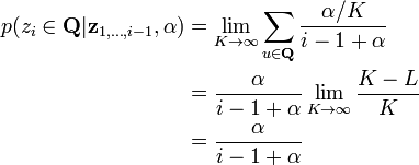
$\begin{align} p(z_i \in \mathbf{Q}|\mathbf{z}_{1,\dots,i-1},\alpha) & = \lim_{K\to\infty} \sum_{u\in\mathbf{Q}} \frac{\alpha/K}{i - 1 + \alpha} \\ &= \frac{\alpha}{i-1+\alpha} \lim_{K\to\infty} \frac{K-L}{K} \\ &= \frac{\alpha}{i-1+\alpha} \end{align}$

In other words:

The probability of seeing an already-seen component is proportional to the number of times that component has been seen.
The probability of seeing any unseen component is proportional to the concentration parameter .

This process is termed a Chinese restaurant process (CRP). In terms of the CRP, the infinite-dimensional model can equivalently be written:

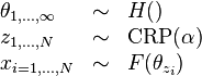
$\begin{array}{lcl} \theta_{1,\dots,\infty} &\sim& H \\ z_{1,\dots,N} &\sim& \operatorname{CRP}(\alpha) \\ x_{i=1,\dots,N} &\sim& F(\theta_{z_i}) \end{array}$

Note that we have marginalized out the mixing probabilities, and thereby produced a more compact representation of the model.

Now imagine further that we also marginalize out the component assignments, and instead we look directly at the distribution of . Then, we can write the model directly in terms of the Dirichlet process:

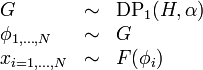
$\begin{array}{lcl} G &\sim& \operatorname{DP}_1(H,\alpha) \\ \phi_{1,\dots,N} &\sim& G \\ x_{i=1,\dots,N} &\sim& F(\phi_i) \end{array}$

represents one view (the distribution-centered view) of the Dirichlet process as producing a random, infinite-dimensional discrete distribution with values drawn from .

An alternative view of the Dirichlet process (the process-centered view), adhering more closely to its definition as a stochastic process, sees it as directly producing an infinite stream of values. Notating this view as, we can write the model as

$\begin{array}{lcl} \phi_{1,\dots} &\sim& \operatorname{DP}_2(H,\alpha) \\ x_{i=1,\dots,N} &\sim& F(\phi_i) \end{array}$

In this view, although the Dirichet process generates an infinite stream of parameter values, we only care about the first N values. Note that some of these values will be the same as previously seen values, in a "rich get richer" scheme, as determined by the Chinese restaurant process.

Read more about this topic: Dirichlet Process

Famous quotes containing the word introduction:

“For better or worse, stepparenting is self-conscious parenting. You’re damned if you do, and damned if you don’t.”
—Anonymous Parent. Making It as a Stepparent, by Claire Berman, introduction (1980, repr. 1986)

“My objection to Liberalism is this—that it is the introduction into the practical business of life of the highest kind—namely, politics—of philosophical ideas instead of political principles.”
—Benjamin Disraeli (1804–1881)

“Such is oftenest the young man’s introduction to the forest, and the most original part of himself. He goes thither at first as a hunter and fisher, until at last, if he has the seeds of a better life in him, he distinguishes his proper objects, as a poet or naturalist it may be, and leaves the gun and fish-pole behind. The mass of men are still and always young in this respect.”
—Henry David Thoreau (1817–1862)