Geometric Mean
The logarithm of the geometric mean of a distribution with random variable X is the arithmetic mean of ln X, or, equivalently, its expected value:
For a beta distribution, the expected value integral gives:

where is the digamma function.
Therefore the geometric mean of a beta distribution with shape parameters α and β is the exponential of the digamma functions of α and β as follows:
While for a beta distribution with equal shape parameters α = β, it follows that skewness = 0 and mode = mean = median = 1/2, the geometric mean is less than 1/2: 0 < < 1/2. The reason for this is that the logarithmic transformation strongly weights the values of X close to zero, as ln X strongly tends towards negative infinity as X approaches zero, while ln X flattens towards zero as X approaches 1.
Along a line α = β, the following limits apply:

Following are the limits with one parameter finite (non zero) and the other approaching these limits:

The accompanying plot shows the difference between the mean and the geometric mean for shape parameters α and β from zero to 2. Besides the fact that the difference between them approaches zero as α and β approach infinity and that the difference becomes large for values of α and β approaching zero, one can observe an evident asymmetry of the geometric mean with respect to the shape parameters α and β. The difference between the geometric mean and the mean is larger for small values of α in relation to β than when exchanging the magnitudes of β and α.
N.L.Johnson and S.Kotz suggest the logarithmic approximation to the digamma function which results in the following approximation to the geometric mean:
Numerical values for the relative error in this approximation follow: ; ; ; ; ; ;; .
Similarly, one can calculate the value of shape parameters required for the geometric mean to equal 1/2. Let's say that we know one of the parameters, β, what would be the value of the other parameter, α, required for the geometric mean to equal 1/2 ?. The answer is that (for β > 1), the value of α required tends towards β + 1/2 as β → ∞. For example, all these couples have the same geometric mean of 1/2:, .
The fundamental property of the geometric mean, which can be proven to be false for any other mean, is
This makes the geometric mean the only correct mean when averaging normalized results, that is results that are presented as ratios to reference values. This is relevant because the beta distribution is a suitable model for the random behavior of percentages and it is particularly suitable to the statistical modelling of proportions. The geometric mean plays a central role in maximum likelihood estimation, see section "Parameter estimation, maximum likelihood." Actually, when performing maximum likelihood estimation, besides the geometric mean based on the random variable X, also another geometric mean appears naturally: the geometric mean based on the linear transformation (1 − X), the mirror-image of X, denoted by :
Along a line α = β, the following limits apply:
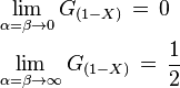
Following are the limits with one parameter finite (non zero) and the other approaching these limits:

It has the following approximate value:
Although both and are asymmetric, in the case that both shape parameters are equal, the geometric means are equal: . This equality follows from the following symmetry displayed between both geometric means:
Read more about this topic: Beta Distribution, Properties, Measures of Central Tendency
Famous quotes containing the word geometric:
“In mathematics he was greater
Than Tycho Brahe, or Erra Pater:
For he, by geometric scale,
Could take the size of pots of ale;
Resolve, by sines and tangents straight,
If bread and butter wanted weight;
And wisely tell what hour o’ th’ day
The clock doth strike, by algebra.”
—Samuel Butler (1612–1680)
“New York ... is a city of geometric heights, a petrified desert of grids and lattices, an inferno of greenish abstraction under a flat sky, a real Metropolis from which man is absent by his very accumulation.”
—Roland Barthes (1915–1980)