Multinomial Probit - Example: Bivariate Probit

Example: Bivariate Probit

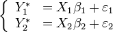
are two binary dependent variables. In the Ordinary Probit model, one latent variable is used, in the bivariate probit model there are two: and . These latent variables are defined as: 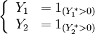$\left\{ \begin{array}{ll} Y_1&=1_{(Y^*_1>0)}\\ Y_2&=1_{(Y^*_2>0)} \end{array} \right.$

with

$\left\{ \begin{array}{ll} Y_1^*&=X_1\beta_1+\varepsilon_1\\ Y_2^*&=X_2\beta_2+\varepsilon_2 \end{array} \right.$

And:

$\left( \begin{array}{c} \varepsilon_1\\ \varepsilon_2 \end{array} \right)|X \sim \mathcal{N} \left(\left( \begin{array}{c} 0\\ 0 \end{array} \right) , \left( \begin{array}{cc} 1&\rho\\ \rho&1 \end{array} \right)\right)$

Fitting the bivariate probit model involves estimating the values of . To do so, the Likelihood of the model has to be maximized. This Likelihood is defined as:

$\prod P(Y_1=1,Y_2=1)^{Y_1Y_2}P(Y_1=0,Y_2=1)^{(1-Y_1)Y_2}P(Y_1=1,Y_2=0)^{Y_1(1-Y_2)}P(Y_1=0,Y_2=0)^{(1-Y_1)(1-Y_2)}$ Substituting the latent variables and in the Probability functions and taking Log's gives: $\sum Y_1Y_2\ln P(\varepsilon_1>-X_1\beta_1,\varepsilon_2>-X_2\beta_2) +(1-Y_1)Y_2\ln P(\varepsilon_1<-X_1\beta_1,\varepsilon_2>-X_2\beta_2) +Y_1(1-Y_2)\ln P(\varepsilon_1>-X_1\beta_1,\varepsilon_2<-X_2\beta_2) +(1-Y_1)(1-Y_2)\ln P(\varepsilon_1<-X_1\beta_1,\varepsilon_2<-X_2\beta_2)$

After some rewriting, the log-likelihood function becomes: $\sum Y_1Y_2\ln \Phi(X_1\beta_1,X_2\beta_2,\rho)+(1-Y_1)Y_2\ln \Phi(-X_1\beta_1,X_2\beta_2,-\rho)+Y_1(1-Y_2)\ln \Phi(X_1\beta_1,-X_2\beta_2,-\rho)+(1-Y_1)(1-Y_2)\ln \Phi(-X_1\beta_1,-X_2\beta_2,\rho)$ Note that is the cumulative distribution function of the bivariate normal distribution. and in the log-likelihood function are observed variables being equal to one or zero.

To maximize the log-likelihood function it is recommended to define the gradient.

Read more about this topic: Multinomial Probit