Land-use Forecasting - Penn-Jersey Model

Penn-Jersey Model

The P-J (Penn-Jersey, greater Philadelphia area) analysis had little impact on planning practice. However, it illustrates what planners might have done, given available knowledge building blocks. It is an introduction to some of the work by researchers who are not practicing planners.

The P-J study scoped widely for concepts and techniques. It scoped well beyond the CATS and Lowry efforts, especially taking advantage of things that had come along in the late 1950s. It was well funded and viewed by the State and the Bureau of Public Roads as a research and a practical planning effort. Its director’s background was in public administration, and leading personnel were associated with the urban planning department at the University of Pennsylvania. The P-J study was planning and policy oriented.

The P-J study drew on several factors "in the air". First, there was a lot of excitement about economic activity analysis and the applied math that it used, at first, linear programming. T. J. Koopmans, the developer of activity analysis, had worked in transportation. There was pull for transportation (and communications) applications, and the tools and interested professionals were available.

There was work on flows on networks, through nodes, and activity location. Orden (1956) had suggested the use of conservation equations when networks involved intermediate modes; flows from raw material sources through manufacturing plants to market were treated by Beckmann and Marschak (1955) and Goldman (1958) had treated commodity flows and the management of empty vehicles.

Maximal flow and synthesis problems were also treated (Boldreff 1955, Gomory and Hu 1962, Ford and Fulkerson 1956, Kalaba and Juncosa 1956, Pollack 1964). Balinski (1960) considered the problem of fixed cost. Finally, Cooper (1963) considered the problem of optimal location of nodes. The problem of investment in link capacity was treated by Garrison and Marble (1958) and the issue of the relationship between the length of the planning time-unit and investment decisions was raised by Quandt (1960) and Pearman (1974).

A second set of building blocks was evolving in location economics, regional science, and geography. Edgar Dunn (1954) undertook an extension of the classic von Thünen analysis of the location of rural land uses. Also, there had been a good bit of work in Europe on the interrelations of economic activity and transportation, especially during the railroad deployment era, by German and Scandinavian economists. That work was synthesized and augmented in the 1930s by August Lösch, and his The Location of Economic Activities was translated into English during the late 1940s. Edgar Hoover’s work with the same title was also published in the late 1940s. Dunn’s analysis was mainly graphical; static equilibrium was claimed by counting equations and unknowns. There was no empirical work (unlike Garrison 1958). For its time, Dunn’s was a rather elegant work.

William Alonso's (1964) work soon followed. It was modeled closely on Dunn’s and also was a University of Pennsylvania product. Although Alonso’s book was not published until 1964, its content was fairly widely known earlier, having been the subject of papers at professional meetings and Committee on Urban Economics (CUE) seminars. Alonso’s work became much more widely known than Dunn’s, perhaps because it focused on “new” urban problems. It introduced the notion of bid rent and treated the question of the amount of land consumed as a function of land rent.

Wingo (1961) was also available. It was different in style and thrust from Alonso and Dunn’s books and touched more on policy and planning issues. Dunn’s important, but little noted, book undertook analysis of location rent, the rent referred to by Marshall as situation rent. Its key equation was:

$R = Y\left( {P - c} \right) - Ytd$

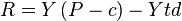
where: R = rent per unit of land, P = market price per unit of product, c = cost of production per unit of product, d = distance to market, and t = unit transportation cost.

In addition, there were also demand and supply schedules.

This formulation by Dunn is very useful, for it indicates how land rent ties to transportation cost. Alonso’s urban analysis starting point was similar to Dunn’s, though he gave more attention to market clearing by actors bidding for space.

The question of exactly how rents tied to transportation was sharpened by those who took advantage of the duality properties of linear programming. First, there was a spatial price equilibrium perspective, as in Henderson (1957, 1958) Next, Stevens (1961) merged rent and transportation concepts in a simple, interesting paper. In addition, Stevens showed some optimality characteristics and discussed decentralized decision-making. This simple paper is worth studying for its own sake and because the model in the P-J study took the analysis into the urban area, a considerable step.

Stevens 1961 paper used the linear programming version of the transportation, assignment, translocation of masses problem of Koopmans, Hitchcock, and Kantorovich. His analysis provided an explicit link between transportation and location rent. It was quite transparent, and it can be extended simply. In response to the initiation of the P-J study, Herbert and Stevens (1960) developed the core model of the P-J Study. Note that this paper was published before the 1961 paper. Even so, the 1961 paper came first in Stevens’ thinking.

The Herbert–Stevens model was housing centered, and the overall study had the view that the purpose of transportation investments and related policy choices was to make Philadelphia a good place to live. Similar to the 1961 Stevens paper, the model assumed that individual choices would lead to overall optimization.

The P-J region was divided into u small areas recognizing n household groups and m residential bundles. Each residential bundle was defined on the house of apartment, the amenity level in the neighborhood (parks, schools, etc.), and the trip set associated with the site. There is an objective function:

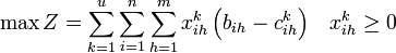
$\max Z = \sum_{k = 1}^u {\sum_{i = 1}^n {\sum_{h = 1}^m {x_{ih}^k \left( {b_{ih} - c_{ih}^k } \right)} } } \quad x_{ih}^k \geq 0$

wherein x_ihk is the number of households in group i selecting residential bundle h in area k. The items in brackets are bih (the budget allocated by i to bundle h) and c_ihk, the purchase cost of h in area k. In short, the sum of the differences between what households are willing to pay and what they have to pay is maximized; a surplus is maximized. The equation says nothing about who gets the surplus: it is divided between households and those who supply housing in some unknown way. There is a constraint equation for each area limiting the land use for housing to the land supply available.

$\sum_{i = 1}^n {\sum_{h = 1}^m {s_{ih} x_{ih}^k } } \leq L^k$

where: s_ih = land used for bundle h L_k = land supply in area k

And there is a constraint equation for each household group assuring that all folks can find housing.

$\sum_{k = 1}^u {\sum_{h = 1}^m {x_{ih}^k } } = N_i$

where: N_i = number of households in group i

A policy variable is explicit, the land available in areas. Land can be made available by changing zoning and land redevelopment. Another policy variable is explicit when we write the dual of the maximization problem, namely:

$\min Z' = \sum_{k = 1}^u {r^k L^k + \sum_{i = 1}^n {v_i \left( { - N_i } \right)} }$

Subject to:

$s_{ih} r^k - v_i \geq b_{ih} - c_{ih}^k$

$r^k \geq 0$

The variables are rk (rent in area k) and v_i an unrestricted subsidy variable specific to each household group. Common sense says that a policy will be better for some than others, and that is reasoning behind the subsidy variable. The subsidy variable is also a policy variable because society may choose to subsidize housing budgets for some groups. The constraint equations may force such policy actions.

It is apparent that the Herbert–Stevens scheme is a very interesting one. Its also apparent that it is housing centered, and the tie to transportation planning is weak. That question is answered when we examine the overall scheme for study, the flow chart of a single iteration of the model. How the scheme works requires little study. The chart doesn’t say much about transportation. Changes in the transportation system are displayed on the chart as if they are a policy matter.

The word “simulate” appears in boxes five, eight, and nine. The P-J modelers would say, “We are making choices about transportation improvements by examining the ways improvements work their way through urban development. The measure of merit is the economic surplus created in housing.”

Academics paid attention to the P-J study. The Committee on Urban Economics was active at the time. The committee was funded by the Ford Foundation to assist in the development of the nascent urban economics field. It often met in Philadelphia for review of the P-J work. Stevens and Herbert were less involved as the study went along. Harris gave intellectual leadership, and he published a fair amount about the study (1961, 1962). However, the P-J influence on planning practice was nil. The study didn’t put transportation up front. There were unsolvable data problems. Much was promised but never delivered. The Lowry model was already available.

Read more about this topic: Land-use Forecasting

Famous quotes containing the word model:

“Research shows clearly that parents who have modeled nurturant, reassuring responses to infants’ fears and distress by soothing words and stroking gentleness have toddlers who already can stroke a crying child’s hair. Toddlers whose special adults model kindliness will even pick up a cookie dropped from a peer’s high chair and return it to the crying peer rather than eat it themselves!”
—Alice Sterling Honig (20th century)