Kalman Filter - Hybrid Kalman Filter

Hybrid Kalman Filter

Most physical systems are represented as continuous-time models while discrete-time measurements are frequently taken for state estimation via a digital processor. Therefore, the system model and measurement model are given by

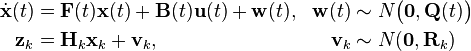
$\begin{align} \dot{\mathbf{x}}(t) &= \mathbf{F}(t)\mathbf{x}(t)+\mathbf{B}(t)\mathbf{u}(t)+\mathbf{w}(t), &\mathbf{w}(t) &\sim N\bigl(\mathbf{0},\mathbf{Q}(t)\bigr) \\ \mathbf{z}_k &= \mathbf{H}_k\mathbf{x}_k+\mathbf{v}_k, &\mathbf{v}_k &\sim N(\mathbf{0},\mathbf{R}_k) \end{align}$

where

Initialize: $\hat{\mathbf{x}}_{0|0}=E\bigl, \mathbf{P}_{0|0}=Var\bigl$
Predict: $\begin{align} &\dot{\hat{\mathbf{x}}}(t) = \mathbf{F}(t) \hat{\mathbf{x}}(t) + \mathbf{B}(t) \mathbf{u}(t) \text{, with } \hat{\mathbf{x}}(t_{k-1}) = \hat{\mathbf{x}}_{k-1|k-1} \\ \Rightarrow &\hat{\mathbf{x}}_{k|k-1} = \hat{\mathbf{x}}(t_k)\\ &\dot{\mathbf{P}}(t) = \mathbf{F}(t)\mathbf{P}(t)+\mathbf{P}(t)\mathbf{F}(t)^T+\mathbf{Q}(t) \text{, with } \mathbf{P}(t_{k-1}) = \mathbf{P}_{k-1|k-1}\\ \Rightarrow &\mathbf{P}_{k|k-1} = \mathbf{P}(t_k) \end{align}$

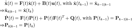
The prediction equations are derived from those of continuous-time Kalman filter without update from measurements, i.e., . The predicted state and covariance are calculated respectively by solving a set of differential equations with the initial value equal to the estimate at the previous step.

Update

The update equations are identical to those of discrete-time Kalman filter.

Read more about this topic: Kalman Filter