BKL Singularity - Oscillating Mode Towards The Singularity

Oscillating Mode Towards The Singularity

The four conditions that had to be imposed on the coordinate functions in the solution eq. 7 are of different types: three conditions that arise from the equations = 0 are "natural"; they are a consequence of the structure of Einstein equations. However, the additional condition λ = 0 that causes the loss of one derivative function, is of entirely different type.

The general solution by definition is completely stable; otherwise the Universe would not exist. Any perturbation is equivalent to a change in the initial conditions in some moment of time; since the general solution allows arbitrary initial conditions, the perturbation is not able to change its character. In other words, the existence of the limiting condition λ = 0 for the solution of eq. 7 means instability caused by perturbations that break this condition. The action of such perturbation must bring the model to another mode which thereby will be most general. Such perturbation cannot be considered as small: a transition to a new mode exceeds the range of very small perturbations.

The analysis of the behavior of the model under perturbative action, performed by BKL, delineates a complex oscillatory mode on approaching the singularity. They could not give all details of this mode in the broad frame of the general case. However, BKL explained the most important properties and character of the solution on specific models that allow far-reaching analytical study.

These models are based on a homogeneous space metric of a particular type. Supposing a homogeneity of space without any additional symmetry leaves a great freedom in choosing the metric. All possible homogeneous (but anisotropic) spaces are classified, according to Bianchi, in 9 classes. BKL investigate only spaces of Bianchi Types VIII and IX.

If the metric has the form of eq. 7, for each type of homogeneous spaces exists some functional relation between the reference vectors l, m, n and the space coordinates. The specific form of this relation is not important. The important fact is that for Type VIII and IX spaces, the quantities λ, μ, ν eq. 10 are constants while all "mixed" products l rot m, l rot n, m rot l, etc. are zeros. For Type IX spaces, the quantities λ, μ, ν have the same sign and one can write λ = μ = ν = 1 (the simultaneous sign change of the 3 constants does not change anything). For Type VIII spaces, 2 constants have a sign that is opposite to the sign of the third constant; one can write, for example, λ = − 1, μ = ν = 1.

The study of the effect of the perturbation on the "Kasner mode" is thus confined to a study on the effect of the λ-containing terms in the Einstein equations. Type VIII and IX spaces are the most suitable models exactly in this connection. Since all 3 quantities λ, μ, ν differ from zero, the condition λ = 0 does not hold irrespective of which direction l, m, n has negative power law time dependence.

The Einstein equations for the Type VIII and Type IX space models are

(eq. 22)

(eq. 23)

(the remaining components, are identically zeros). These equations contain only functions of time; this is a condition that has to be fulfilled in all homogeneous spaces. Here, the eq. 22 and eq. 23 are exact and their validity does not depend on how near one is to the singularity at t = 0.

The time derivatives in eq. 22 and eq. 23 take a simpler form if а, b, с are substituted by their logarithms α, β, γ:

(eq. 24)

substituting the variable t for τ according to:

(eq. 25)

Then:

(eq. 26)

(eq. 27)

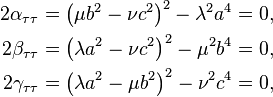
Adding together equations eq. 26 and substituting in the left hand side the sum (α + β + γ)_{τ τ} according to eq. 27, one obtains an equation containing only first derivatives which is the first integral of the system eq. 26:

(eq. 28)

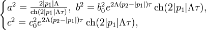
This equation plays the role of a binding condition imposed on the initial state of eq. 26. The Kasner mode eq. 8 is a solution of eq. 26 when ignoring all terms in the right hand sides. But such situation cannot go on (at t → 0) indefinitely because among those terms there are always some that grow. Thus, if the negative power is in the function a(t) (p_l = p₁) then the perturbation of the Kasner mode will arise by the terms λ2a4; the rest of the terms will decrease with decreasing t. If only the growing terms are left in the right hand sides of eq. 26, one obtains the system:

(eq. 29)

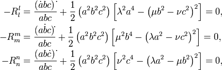
(compare eq. 16; below it is substituted λ2 = 1). The solution of these equations must describe the metric evolution from the initial state, in which it is described by eq. 8 with a given set of powers (with p_l < 0); let p_l = р₁, p_m = р₂, p_n = р₃ so that

(eq. 30)

Then

(eq. 31)

where Λ is constant. Initial conditions for eq. 29 are redefined as

(eq. 32)

Equations eq. 29 are easily integrated; the solution that satisfies the condition eq. 32 is

(eq. 33)

where b₀ and c₀ are two more constants.

It can easily be seen that the asymptotic of functions eq. 33 at t → 0 is eq. 30. The asymptotic expressions of these functions and the function t(τ) at τ → −∞ is

Expressing a, b, c as functions of t, one has

(eq. 34)

where

(eq. 35)

Then

(eq. 36)

The above shows that perturbation acts in such way that it changes one Kasner mode with another Kasner mode, and in this process the negative power of t flips from direction l to direction m: if before it was p_l < 0, now it is p'_m < 0. During this change the function a(t) passes through a maximum and b(t) passes through a minimum; b, which before was decreasing, now increases: a from increasing becomes decreasing; and the decreasing c(t) decreases further. The perturbation itself (λ2a4α in eq. 29), which before was increasing, now begins to decrease and die away. Further evolution similarly causes an increase in the perturbation from the terms with μ2 (instead of λ2) in eq. 26, next change of the Kasner mode, and so on.

It is convenient to write the power substitution rule eq. 35 with the help of the parametrization eq. 5:

(eq. 37)

The greater of the two positive powers remains positive.

BKL call this flip of negative power between directions a Kasner epoch. The key to understanding the character of metric evolution on approaching singularity is exactly this process of Kasner epoch alternation with flipping of powers p_l, p_m, p_n by the rule eq. 37.

The successive alternations eq. 37 with flipping of the negative power p₁ between directions l and m (Kasner epochs) continues by depletion of the whole part of the initial u until the moment at which u < 1. The value u < 1 transforms into u > 1 according to eq. 6; in this moment the negative power is p_l or p_m while p_n becomes the lesser of two positive numbers (p_n = p₂). The next series of Kasner epochs then flips the negative power between directions n and l or between n and m. At an arbitrary (irrational) initial value of u this process of alternation continues unlimited.

In the exact solution of the Einstein equations, the powers p_l, p_m, p_n lose their original, precise, sense. This circumstance introduces some "fuzziness" in the determination of these numbers (and together with them, to the parameter u) which, although small, makes meaningless the analysis of any definite (for example, rational) values of u. Therefore, only these laws that concern arbitrary irrational values of u have any particular meaning.

The larger periods in which the scales of space distances along two axes oscillate while distances along the third axis decrease monotonously, are called eras; volumes decrease by a law close to ~ t. On transition from one era to the next, the direction in which distances decrease monotonously, flips from one axis to another. The order of these transitions acquires the asymptotic character of a random process. The same random order is also characteristic for the alternation of the lengths of successive eras (by era length, BKL understand the number of Kasner epoch that an era contains, and not a time interval).

The era series become denser on approaching t = 0. However, the natural variable for describing the time course of this evolution is not the world time t, but its logarithm, ln t, by which the whole process of reaching the singularity is extended to −∞.

According to eq. 33, one of the functions a, b, c, that passes through a maximum during a transition between Kasner epochs, at the peak of its maximum is

(eq. 38)

where it is supposed that a_max is large compared to b₀ and c₀; in eq. 38 u is the value of the parameter in the Kasner epoch before transition. It can be seen from here that the peaks of consecutive maxima during each era are gradually lowered. Indeed, in the next Kasner epoch this parameter has the value u' = u − 1, and Λ is substituted according to eq. 36 with Λ' = Λ(1 − 2|p₁(u)|). Therefore, the ratio of 2 consecutive maxima is

and finally

(eq. 39)

The above are solutions to Einstein equations in vacuum. As for the pure Kasner mode, matter does not change the qualitative properties of this solution and can be written into it disregarding its reaction on the field.

However, if one does this for the model under discussion, understood as an exact solution of the Einstein equations, the resulting picture of matter evolution would not have a general character and would be specific for the high symmetry imminent to the present model. Mathematically, this specificity is related to the fact that for the homogeneous space geometry discussed here, the Ricci tensor components are identically zeros and therefore the Einstein equations would not allow movement of matter (which gives non-zero stress energy-momentum tensor components ).

This difficulty is avoided if one includes in the model only the major terms of the limiting (at t → 0) metric and writes into it a matter with arbitrary initial distribution of densities and velocities. Then the course of evolution of matter is determined by its general laws of movement eq. 17 and eq. 18 that result in eq. 21. During each Kasner epoch, density increases by the law

(eq. 40)

where p₃ is, as above, the greatest of the numbers p₁, p₂, p₃. Matter density increases monotonously during all evolution towards the singularity.

To each era (s-th era) correspond a series of values of the parameter u starting from the greatest, and through the values − 1, − 2, ..., reaching to the smallest, < 1. Then

(eq. 41)

that is, k(s) = where the brackets mean the whole part of the value. The number k(s) is the era length, measured by the number of Kasner epochs that the era contains. For the next era

(eq. 42)

In the limiteless series of numbers u, composed by these rules, there are infinitesimally small (but never zero) values x(s) and correspondingly infinitely large lengths k(s).